Twittering about climate change and Bangladesh

Points of post:

• To describe how twitteR can be used, together with Word Clouds (wordcloud), to reveal what people are twittering about.
• To show how rapidly interest in various subjects can change.

Twitter (https://twitter.com/) is a social media network allowing users to send short (140 characters) messages called ‘tweets’. Twitter started up in 2006 and has had phenomenal success with 340 million tweets sent each day in 2012. 

In an earlier post on our blog, we described how archives of Google internet searches can tell us what people are interested in, and how these interests change over time. It is also possible to assess what factors might be affecting this interest, e.g. a disease outbreak or climatic disaster. Similarly Twitter might be viewed as a massive, passive opinion poll. 

Again wonderful R has libraries to analyze the worlds’ tweets (twitteR) which can be useful to perform social media mining and to reveal what people are thinking (twittering) about; whether it’s Brad Pitts’ facial hair (http://www.dailymail.co.uk/tvshowbiz/article-2792839/brad-pitt-continues-wear-rakish-moustache-long-sideburns-grew-sea-new-york.html) or climate variability and change. 

Jason and I are very interested in how climate change will affect the people of Bangladesh, in particular, and we’ve already explored the temporal and spatial dependence of various weather variables such as temperature and sea-level in the country. 

Hence we experimented by inserting the two keywords, ‘climate-change’ and ‘Bangladesh’ as our search parameters into twitteR. Our aim was to reveal with what other words or phrases these keywords were associated. ‘Word Clouds’ are a useful way to summarize the results. In Word cloud graphical representations, font sizes are scaled according to the frequencies at which words occur; in this case how often they are ‘tweeted’. Below is a Word cloud for September 2014 which shows that ‘URBANISATION’ and ‘ROUND TABLE’ occurred most often in tweets.

By December 2014, however, when we tried again, the identical keywords were associated with ‘FLOATING GARDENS’, and the increasingly nebulous ‘ADAPTATION’ and ‘RESILIENCE’.

Clearly social media such as Twitter, combined with R’s software packages and plotting facilities, are fantastic tools for understanding the often capricious winds affecting the movement of global public interest and opinion.

To carry out your own social media mining using the twitteR package, you will first need to have an account on twitter and create an 'app'. Please see this and this link to get a better idea on how to get that done.

You will also find information in the above links on the 'twitter authentication' process which is also required to be able to perform the keyword searches using twitteR.

The code used to produce the above word clouds is outlined below.

# Load required libraries

library(RCurl)
library(stringr)
library(tm)
library(wordcloud)
library(RColorBrewer)
library(twitteR)
library(streamR)
library(grid)
library(ggplot2)
library(wesanderson)
 
# Load credentials
load("D:/ClimData/Twitter/twitter authentification.Rdata")
registerTwitterOAuth(twitCred)
options(RCurlOptions = list(cainfo = system.file("CurlSSL", "cacert.pem", package = "RCurl")))
 
tweets <- searchTwitter("Climate Change Bangladesh", n=1500, lang="en") 
 
tweets.text <- sapply(tweets, function(x) x$getText())
 
# Remove non alphanumeric characters
tweets.text <- gsub("[^a-zA-Z0-9 ]","",tweets.text)
 
# Convert all text to lower case
tweets.text <- tolower(tweets.text)
 
# Replace blank space (“rt”)
tweets.text <- gsub("rt", "", tweets.text)
 
# Replace @UserName
tweets.text <- gsub("@\\w+", "", tweets.text)
 
# Remove punctuation
tweets.text <- gsub("[[:punct:]]", "", tweets.text)
 
# Remove links
tweets.text <- gsub("http\\w+", "", tweets.text)
 
# Remove tabs
tweets.text <- gsub("[ |\t]{2,}", "", tweets.text)
 
# Remove blank spaces at the beginning
tweets.text <- gsub("^ ", "", tweets.text)
 
# Remove blank spaces at the end
tweets.text <- gsub(" $", "", tweets.text)
 
# remove word amp
tweet.text <- gsub("amp","",tweets.text)
 
# Create corpus
tweets.text.corpus <- Corpus(VectorSource(tweets.text))
 
# Clean up by removing stop words
tweets.text.corpus <- tm_map(tweets.text.corpus, function(x)removeWords(x,stopwords()))
 
# Create document term matrix applying some transformations
tdm = TermDocumentMatrix(tweets.text.corpus,
      control = list(removePunctuation = TRUE,
      stopwords = c("climate change","bangladesh","climate", "change"), stopwords("english"),
      removeNumbers = TRUE, tolower = TRUE))
 
# Define tdm as matrix
m = as.matrix(tdm)
 
# Get word counts in decreasing order
word_freqs = sort(rowSums(m), decreasing=TRUE) 
 
# Create a data frame with words and their frequencies
dm = data.frame(word=names(word_freqs), freq=word_freqs)
 
# Plot and save the image in png format
png("BGD_ClimateChange_Dec2014.png", width=5, height=5, units="in", res=500)
 
wordcloud(dm$word, dm$freq, random.order=FALSE, min.freq = 2,scale=c(4,0.5),max.words = 100,colors=wes.palette(5,"Darjeeling"))
 
dev.off()

Created by Pretty R at inside-R.org

Come hell with high water - Sea level rises at two stations in Bangladesh

Key points of post

• Bangladesh is low-lying
• Many people live along its river and coasts
• These communities are vulnerable to rises in sea-level which is predicted to occur as a consequence of climate change

Coastal Bangladesh is extremely low-lying and its coastal communities in particular are vulnerable from any future rises in sea level which can cause flooding. Jason and I wondered, therefore, if there were any time-series on sea-level for Bangladesh available, and what information they might contain.

Via Google we discovered the University of Hawaii Sea Level Centre, which monitors seawater levels at stations throughout the world, exploiting its network and relationships with a range of local partners.  In this case it’s the Bangladesh Inland Water Transport Authority who provided the original data.

Here we plot average daily sea level available on the UHSLC site for two stations (please map below) at Charchanga (at the mouth of the Meghna River) and Hiron Point (in the Sundarbans). [Note there are data for 5 other stations in Bangladesh but the time-series data available were, unfortunately, too short a duration]. The data are also color-coded to correspond to the six seasons of Bangladesh (winter, spring, summer, monsoon, autumn, & late autumn). 

Data: stations.google • Chart ID: MapID1f246f024be6 • googleVis-0.5.6
R version 3.1.2 (2014-10-31) • Google Terms of Use • Documentation and Data Policy

The first interesting feature, noted at both locations, is the pronounced seasonality with peaks in sea-level being recorded in the  monsoon, autumn and late autumn periods.  Winter and spring correspond to lowest average daily water levels at both locations.  The seasonal variation in sea-level is due primarily to the effect of the Monsoon; ie. the south-westerly winds tend to cause the seas to ‘pile-up’ along the coast of Bangladesh, while the flow from the major rivers pouring through the delta into the Bay of Bengal increases substantially also as a result of the Monsoon. 

The most worrying aspect of these data is the substantial change in long-term trend summarized here with a simple linear model (red line).  At Charchanga average daily sea-levels recorded rose by approximately 7 mm's per year between 1980 and 2000 while at Hiron Point the figure was approximately 5 mm's per year (1977 to 2003). Unfortunately more recent data were unavailable from the Sea Level Center and we are currently unsure if these trends are continuing. But please if you know of more data for Bangladesh let us know.

Certain aspects of the series are, however, rather curious and it’s not a straightforward story of increasing trends.  At Hiron Point, for example, extreme sea-level events (say above 2600 mm's) were relatively frequently between 1980 and 1995 whereas, since 1996 they have been observed less often. Contrast this with Charchanga where there were some exceptional peaks recorded in 1996, ’97, and ’98. 

All such changes could have profound implications for the livelihoods of coastal Bangladeshis.

Details of how to obtain the data and plot the graphs here in R are demonstrated below.  

As mentioned earlier in the post, the data was obtained from the University of Hawaii Sea Level Centre and we have used the research quality dataset which can be found at this link - http://uhslc.soest.hawaii.edu/data/download/rq

You can download the dataset in various formats which include csv and NetCDF and the associated metadata for each station is also there for you to check of any inconsistencies in the data collection or station relocation and instrumentation issues. The data can also be downloaded at two different time scales, which is hourly and daily. 

# Load required libraries
 
library(ggplot2)
library(scales)
library(grid)
library(plyr)
library(lubridate)
library(zoo)
 
# Set working directory
 
setwd("D:/ClimData/SeaLevel")
 
# Read csv file
 
sl<-read.csv("rqd0138a.csv",header=FALSE)
 
# Rename columns
 
colnames(sl)<-c("year","month","day","sl_mm")
 
# Format date columns
 
sl$date <- as.Date(paste(sl$year,sl$month,sl$day),format="%Y%m%d")
sl$month <- as.numeric(format(sl$date,"%m"))
sl$year <- as.numeric(format(sl$date,"%Y"))
sl$monthf <- factor(sl$month,levels=as.character(1:12),labels=c("Jan","Feb","Mar","Apr","May","Jun","Jul","Aug","Sep","Oct","Nov","Dec"),ordered=TRUE)
sl$mday <- strptime(sl$date, "%Y-%m-%d")$mday
sl$jday <- strptime(sl$date, "%Y-%m-%d")$yday+1
sl$daymth <- as.character(paste(sl$month,sl$day,sep="-"))
sl$daymth <-as.Date(sl$daymth,format="%m-%d")
 
# Classify data into seasons
 
sl$season <- "Season"
 
sl$season[sl$month == 1 & sl$mday >= 1 |  sl$month == 2 & sl$mday <= 13| sl$month == 1]<-'Winter'
sl$season[sl$month == 2 & sl$mday >= 14 |  sl$month == 4 & sl$mday <= 14 | sl$month == 3]<-'Spring'
sl$season[sl$month == 4 & sl$mday >= 15 |  sl$month == 6 & sl$mday <= 14 | sl$month == 5]<-'Summer'
sl$season[sl$month == 6 & sl$mday >= 15 |  sl$month == 8 & sl$mday <= 17 | sl$month == 7]<-'Monsoon'
sl$season[sl$month == 8 & sl$mday >= 18 |  sl$month == 10 & sl$mday <= 18| sl$month == 9]<-'Autumn'
sl$season[sl$month == 10 & sl$mday >= 19 |  sl$month == 12 & sl$mday <= 16| sl$month == 11]<-'Late Autumn'
sl$season[sl$month == 12 & sl$mday >= 17 |  sl$month == 12 & sl$mday <= 31| sl$month == 1]<-'Winter'
 
sl$season = factor(sl$season, c("Winter", "Spring", "Summer", "Monsoon","Autumn","Late Autumn"))
 
## Plot Sea Level
 
hp_sl <-   ggplot(sl, aes(date, sl_mm,colour=season))+
           #geom_line(size=0.5)+
           geom_point(shape=5,size=1)+
           geom_smooth(method="lm",size=0.5,col="red")+
           scale_x_date(name="\n\n\n Source: University of Hawaii Sea Level Centre / Bangladesh Inland Water Transport Authority (BIWTA) - 2014",labels=date_format("%Y"),breaks = date_breaks("2 years"))+
           ylab("Milimetres (mm)\n")+
           xlab("\nYear")+
           theme_bw()+
           ggtitle("Sea Level at Charchanga - Bangladesh (1980-2000)\n")+
           theme(plot.title = element_text(lineheight=1.2, face="bold",size = 14, colour = "grey20"),
           panel.border = element_rect(colour = "black",fill=F,size=1),
           panel.grid.major = element_line(colour = "grey",size=0.25,linetype='longdash'),
           panel.grid.minor = element_blank(),
           axis.title.y=element_text(size=11,colour="grey20"),
           axis.title.x=element_text(size=9,colour="grey20"),
           panel.background = element_rect(fill = NA,colour = "black"))
 
hp_sl
 
# Get gradient and add to plot
 
m <- lm(sl_mm~year, data=sl )
ms <- summary(m)
 
slope <- coef(m)[2]
lg <- list(slope = format(slope, digits=3))
eq <- substitute(italic(Gradient)==slope,lg)
eqstr <-as.character(paste(as.expression(eq),"/year"))
hp_sl <- hp_sl + annotate(geom="text",as.Date(-Inf, origin = '1970-01-01'), y = Inf, 
         hjust = -0.1, vjust = 2, label = eqstr,parse = TRUE,size=3)
 
hp_sl
 
# Save plot to png
 
ggsave(hp_sl, file="Charchanga_SeaLevel_Plot_Seasons.png", width=10, height=6,dpi=400,unit="in",type="cairo")
 
# Code to produce html code of embedded sea level stations map using googleVis
 
# Load libraries
 
library(RCurl)
library(XML)
library(leafletR)
library(googleVis)
 
# Convert html table into data frame
 
theurl <- "http://uhslc.soest.hawaii.edu/data/download/rq"
tables <- readHTMLTable(theurl)
n.rows <- unlist(lapply(tables, function(t) dim(t)[1]))
 
tbl <- tables[[which.max(n.rows)]]
 
bgd.tbl <- subset(tbl, Country =="Bangladesh")
 
bgd.tbl$Latitude <- as.numeric(levels(bgd.tbl$Latitude)[bgd.tbl$Latitude])
bgd.tbl$Longitude <- as.numeric(levels(bgd.tbl$Longitude)[bgd.tbl$Longitude])
 
google.location <- paste(bgd.tbl$Latitude, bgd.tbl$Longitude, sep = ":")
stations.google <- data.frame(bgd.tbl, google.location)
 
# Plot map
 
map <- gvisMap(data = stations.google, locationvar = "google.location",tipvar = "Location",
       options=list(showTip=TRUE, enableScrollWheel=TRUE,mapType='terrain', useMapTypeControl=TRUE,width=100,height=400,
       icons=paste0("{","'default': {'normal': 'http://i.imgur.com/f3q6Oaj.gif',\n",
       "'selected': 'http://i.imgur.com/f3q6Oaj.gif'","}}")))
 
plot(map)

Created by Pretty R at inside-R.org

Climate variability and change: hot air from Bangladesh?

Key points of post

• Here we analyse air temperature from 3 weather stations along a north-south transect in Bangladesh (Rangpur (1982-2013), Dhaka (1998-2013) and Barisal (1998-2013).
• Air temperatures risen at all 3 stations;  Dhaka had the most substantial increases in temperature rising 0.64°C overall between 1998 and 2013.
• Seasonality in temperature varies between years but differences overall are slight and there seems to be no systematic changes in shape.

In this blog post, we ask whether air temperatures are rising in Bangladesh using data available to us from the internet. 

Bangladesh is a beautiful, semi-tropical country with India to the north and west and Myanmar to the east. The country is intersected by vast rivers, fed by the mountains of the Himalayas, which meander through the countryside. The normal seasonal cycles of flooding of these rivers regulates food production in many ways, e.g. irrigating rice or triggering fish production. Bangladesh is mostly low-lying and potentially vulnerable to sea-level rise and cyclones. The country is developing rapidly but much of its population remains poor, clinging to precarious livelihoods around rivers, lakes, and the sea.

Location of Rangpur, Dhaka and Barisal Weather Stations - Bangladesh

Bangladesh is a focal country for our CCAFS program which researches the impact of changing climate and weather on food production in developing countries; and particularly on the consequences for the poorest members of society.  Temperature is a ‘master’ variable, ultimately controlling all life in our biosphere including food production, species distributions and pathogen activity.

Here we examine long-term trends in temperature from the 3 following stations in Bangladesh: Rangpur; Dhaka; and Barisal (see map above). Unfortunately, compared to many other countries, data available for Bangladesh are rather sparse. Even for the capital city of Dhaka, we could only find continuous data from 1998, and there are also substantial gaps. The longest series available to us was from Rangpur which extended 32 years in total from 1982 to 2013. Air temperatures for the 3 stations are plotted below both as simple time-series and 3D, ‘heat-map’ plots, the latter being useful for showing how seasonality changes over longer term time.

The red lines in the 3 time-series plots represent linear models fitted to the data (for all 3 stations) as functions of year. The value of the gradient term (amount of rise/amount of tread) is indicated at the top-left. The gradients were positive in all 3 stations, meaning that temperatures indeed rose but the magnitude of increase is extremely slight compared to other locations we have examined, e.g. in Penang, Malaysia air temperature increases have been comparatively substantial. At Rangpur temperatures rose at 0.0117°C per year over 32 years which means an overall increase of 0.37°C overall (0.0117 x 32). Data were available for shorter periods at Dhaka and Barisal which recorded overall rises of 0.33°C and 0.64°C respectively. In Rangpur, extreme high temperatures (ie. > 35°C) occurred more frequently in the past, between 1982 and 1995, than would be the case for the present (see time-series above). Seasonality indeed varies from year to year (heat-map plots) but there is little evidence of the systematic changes over time that we have seen in other locations. 

The shape of the seasonal cycle seemed to vary only slightly between locations (see below). There is a clear Northern Hemisphere winter, summer cycle with lowest temperatures in December and January. In 2013, Dhaka was on average the warmest of all 3 locations, with peak temperatures occurring in June and July. Barisal was slightly warmer than Rangpur in the early part of the year after when Barisal fell relative to Rangpur. Peak temperatures in all 3 locations occurred (on average between June and July.

The results from these analyses are curious and possibly at odds with the view that the impacts of climate change on Bangladesh are especially worrying.  A rise of 0.64°C between 1998 and 2013 which we see at Dhaka is substantial, whereas further north at Rangpur we only saw a 0.37°C overall increase between 1982 and 2013.  In our view it is unlikely that these rises are even perceptible to the average human, and are also unlikely to have had much impact on food production.

Close examination of actual data can often challenge ‘accepted wisdom’, which is a particular purpose of these articles.  Of course, temperature is just one variable and Bangladesh’s climate future will also depend on the interaction between temperature and other variables such as rainfall and wind speed. Sea-level rise will also be a factor to consider. These will from the subject of future investigations.

The R code used to produce the plots in this blog post is provided below and the datasets used here are from NOAA National Climatic Data Centre's (NCDC) Integrated Surface Database.

# Load required libraries
 
library(ggplot2)
library(scales)
library(grid)
library(plyr)
library(lubridate)
library(zoo)
 
# Set working directory
 
setwd("D:/ClimData/BGD")
 
################################
## Plot Air Temps for Rangpur ##
################################
 
dat <- read.table("826316390028dat.txt",header=TRUE,fill=TRUE,
       na.strings=c("*","**","***","****","*****","******","0.00T*****","0.00T**","0.00T"))
 
colnames(dat)<-tolower(colnames(dat))
 
Sys.setenv(TZ = "UTC")
dat$dates <- as.POSIXct(strptime(dat$yr..modahrmn,format="%Y%m%d%H%M"))  + 6 * 60 * 60
 
dat$tempc <- (dat$temp-32) * (5/9)
 
dat$date <- as.Date(dat$dates,format="%Y%m%d")
 
dat$year <- as.numeric(format(dat$dates,"%Y"))
 
dat$month <- as.numeric(format(dat$dates,"%m"))
 
dat$hour  <- as.numeric(format(dat$dates,"%H"))
 
dat$week  <- as.numeric(format(dat$dates,"%W"))
 
dat$monthf <- factor(dat$month,levels=as.character(1:12),
              labels=c("Jan","Feb","Mar","Apr","May","Jun","Jul","Aug","Sep","Oct","Nov","Dec"),ordered=TRUE)
 
# Chuck out data that is < 0 and > 45
 
dat <- dat[dat$tempc > 0 & dat$tempc < 50, ]
 
datb<-subset(dat, year >= 1982 & year <= 2013)
 
plot.title = 'Daily Air Temperatures in Rangpur (1982-2013)'
plot.subtitle = 'Data source: Integrated Surface Database (ISD) - National Climatic Data Centre (NCDC)'
 
b <- ggplot(data=datb, aes(x=dates, y=tempc)) +
     geom_jitter(colour="grey40",size=1.5,alpha=0.4) +
     scale_y_continuous(breaks=c(10,15,20,25,30,35,40)) +
     theme_bw()+
     scale_x_datetime(breaks = "5 year", minor_breaks = "5 year", labels=date_format("%Y")) +
     xlab("") + ylab(as.expression(expression( paste("Temperature (", degree,"C)") ))) +
     ggtitle(bquote(atop(.(plot.title), atop(italic(.(plot.subtitle)), "")))) +
     theme(plot.title = element_text(face = "bold",size = 16,colour="black")) +
     geom_smooth(aes(group = 1), method = "lm",size=0.75,colour="red")
 
b
 
# Get linear equation value and gradient term
 
m <- lm(tempc~year, data=datb )
ms <- summary(m)
 
slope <- coef(m)[2]
 
lg <- list(slope = format(slope, digits=3))
 
eqg <- substitute(italic(Gradient)==slope,lg)
 
eqgstr <-as.character(as.expression(eqg))
 
# Add gradient term value to plot
 
b <- b +annotate(geom="text",as.POSIXct(-Inf, origin = '1970-01-01'), y = Inf, 
                      hjust = -0.1, vjust = 2, label = eqgstr,parse = TRUE,size=3.5)
 
b
 
col<-c("blue","green","yellow","orange","red")
 
wt <- ggplot(data=datb,aes(x=year,y=week,fill=tempc))+ geom_tile(colour=NA,size=0.65)+
      theme_bw()+
      scale_fill_gradientn(colours=col,name=as.expression(expression( paste("Temperature (", degree,"C)"))))+
      coord_equal(ratio=0.2)+
      ylab("WEEK OF YEAR\n")+
      xlab("\nYEAR\n\nSource: Integrated Surface Database (ISD) - National Climatic Data Centre (NCDC)")+
      scale_x_continuous(expand = c(0,0),breaks = seq(1982, 2015, 2)) +
      scale_y_discrete(expand = c(0,0),breaks = seq(0,52,4))+
      ggtitle("Average weekly air temperatures in Rangpur\n")+
      theme(panel.background=element_rect(fill="grey90"),
      panel.border=element_rect(colour="white"),
      axis.title.y=element_text(size=10,colour="grey20"),
      axis.title.x=element_text(size=10,colour="grey20"),
      axis.text.y=element_text(size=10,colour="grey20",face="bold"),
      axis.text.x=element_text(size=10,colour="grey20",face="bold"),
      plot.title = element_text(lineheight=1.2, face="bold",size = 14, colour = "grey20"),
      panel.grid.major = element_blank(),
      panel.grid.minor = element_blank(),
      legend.key.width=unit(c(0.1,0.1),"in"))
 
wt
 
# Exporting file to png
 
ggsave(b, file="Rangpur_AT_Plot.png", width=10, height=6,dpi=400,unit="in",type="cairo")
 
ggsave(wt, file="Rangpur_AT_HeatMap_Plot.png", width=15, height=6,dpi=400,unit="in",type="cairo")
 
 
##############################
## Plot Air Temps for Dhaka ##
##############################
 
dat <-read.table("820756390032dat.txt",header=TRUE,fill=TRUE,
      na.strings=c("*","**","***","****","*****","******","0.00T*****","0.00T**","0.00T"))
 
colnames(dat)<-tolower(colnames(dat))
 
Sys.setenv(TZ = "UTC")
dat$dates <- as.POSIXct(strptime(dat$yr..modahrmn,format="%Y%m%d%H%M"))  + 6 * 60 * 60
 
dat$tempc <- (dat$temp-32) * (5/9)
 
dat$year <- as.numeric(format(dat$dates,"%Y"))
 
dat$month <- as.numeric(format(dat$dates,"%m"))
 
dat$hour  <- as.numeric(format(dat$dates,"%H"))
 
dat$week  <- as.numeric(format(dat$dates,"%W"))
 
dat$monthf <- factor(dat$month,levels=as.character(1:12),
              labels=c("Jan","Feb","Mar","Apr","May","Jun","Jul","Aug","Sep","Oct","Nov","Dec"),ordered=TRUE)
 
# Chuck out data that is < 0 and > 45
 
dat <- dat[dat$tempc > 0 & dat$tempc < 50, ]
 
datb <- subset(dat, year >= 1998 & year <= 2013)
 
plot.title = 'Daily Air Temperatures in Dhaka (1998-2013)'
plot.subtitle = 'Data source: Integrated Surface Database (ISD) - National Climatic Data Centre (NCDC)'
 
b <- ggplot(data=datb, aes(x=dates, y=tempc)) +
     geom_jitter(colour="grey40",size=1.5,alpha=0.4) +
     scale_y_continuous(breaks=c(10,15,20,25,30,35,40)) +
     theme_bw()+
     scale_x_datetime(breaks = "1 year", minor_breaks = "1 year", labels=date_format("%Y"))  +
     xlab("") + ylab(as.expression(expression( paste("Temperature (", degree,"C)") ))) +
     ggtitle(bquote(atop(.(plot.title), atop(italic(.(plot.subtitle)), "")))) +
     theme(plot.title = element_text(face = "bold",size = 16,colour="black")) +
     geom_smooth(aes(group = 1), method = "lm",size=0.75,colour="red")
 
b
 
# Get linear equation value and gradient term
 
m <- lm(tempc~year, data=datb )
ms <- summary(m)
 
slope <- coef(m)[2]
 
lg <- list(slope = format(slope, digits=3))
 
eqg <- substitute(italic(Gradient)==slope,lg)
 
eqgstr <-as.character(as.expression(eqg))
 
# Add gradient term value to plot
 
b <- b +annotate(geom="text",as.POSIXct(-Inf, origin = '1970-01-01'), y = Inf, 
                 hjust = -0.1, vjust = 2, label = eqgstr,parse = TRUE,size=3.5)
 
b
 
col<-c("blue","green","yellow","orange","red")
 
wt <- ggplot(data=datb,aes(x=year,y=week,fill=tempc))+ geom_tile(colour=NA,size=0.65)+
      theme_bw()+
      scale_fill_gradientn(colours=col,name=as.expression(expression( paste("Temperature (", degree,"C)"))))+
      coord_equal(ratio=0.15)+
      ylab("WEEK OF YEAR\n")+
      xlab("\nYEAR\n\nSource: Integrated Surface Database (ISD) - National Climatic Data Centre (NCDC)")+
      scale_x_continuous(expand = c(0,0),breaks = seq(1998, 2015,1)) +
      scale_y_discrete(expand = c(0,0),breaks = seq(0,52,4))+
      ggtitle("Average weekly air temperatures in Dhaka\n")+
      theme(panel.background=element_rect(fill="grey90"),
      panel.border=element_rect(colour="white"),
      axis.title.y=element_text(size=10,colour="grey20"),
      axis.title.x=element_text(size=10,colour="grey20"),
      axis.text.y=element_text(size=10,colour="grey20",face="bold"),
      axis.text.x=element_text(size=10,colour="grey20",face="bold"),
      plot.title = element_text(lineheight=1.2, face="bold",size = 14, colour = "grey20"),
      panel.grid.major = element_blank(),
      panel.grid.minor = element_blank(),
      legend.key.width=unit(c(0.1,0.1),"in"))
 
wt
 
# Exporting file to png
 
ggsave(b, file="Dhaka_AT_Plot.png", width=10, height=6,dpi=400,unit="in",type="cairo")
 
ggsave(wt, file="Dhaka_AT_HeatMap_Plot.png", width=10, height=5,dpi=400,unit="in",type="cairo")
 
 
################################
## Plot Air Temps for Barisal ##
################################
 
dat <- read.table("8998396389910dat.txt",header=TRUE,fill=TRUE,
       na.strings=c("*","**","***","****","*****","******","0.00T*****","0.00T**","0.00T"))
 
colnames(dat)<-tolower(colnames(dat))
 
Sys.setenv(TZ = "UTC")
dat$dates <- as.POSIXct(strptime(dat$yr..modahrmn,format="%Y%m%d%H%M"))  + 6 * 60 * 60
 
dat$tempc <- (dat$temp-32) * (5/9)
 
dat$year <- as.numeric(format(dat$dates,"%Y"))
 
dat$month <- as.numeric(format(dat$dates,"%m"))
 
dat$hour  <- as.numeric(format(dat$dates,"%H"))
 
dat$week  <- as.numeric(format(dat$dates,"%W"))
 
dat$monthf <- factor(dat$month,levels=as.character(1:12),
              labels=c("Jan","Feb","Mar","Apr","May","Jun","Jul","Aug","Sep","Oct","Nov","Dec"),ordered=TRUE)
 
# Chuck out data that is < 0 and > 45
 
dat <- dat[dat$tempc > 0 & dat$tempc < 50, ]
 
datb<-subset(dat, year >= 1998 & year <= 2013)
 
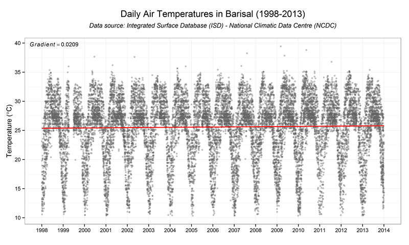
plot.title = 'Daily Air Temperatures in Barisal (1998-2013)'
plot.subtitle = 'Data source: Integrated Surface Database (ISD) - National Climatic Data Centre (NCDC)'
 
b <- ggplot(data=datb, aes(x=dates, y=tempc)) +
     geom_jitter(colour="grey40",size=1.5,alpha=0.4) +
     scale_y_continuous(breaks=c(10,15,20,25,30,35,40)) +
     theme_bw()+
     scale_x_datetime(breaks = "1 year", minor_breaks = "1 year", labels=date_format("%Y"))  +
     xlab("") + ylab(as.expression(expression( paste("Temperature (", degree,"C)") ))) +
     ggtitle(bquote(atop(.(plot.title), atop(italic(.(plot.subtitle)), "")))) +
     theme(plot.title = element_text(face = "bold",size = 16,colour="black"))+
     geom_smooth(aes(group = 1), method = "lm",size=0.75,colour="red")
 
b
 
# Get linear equation value and gradient term
 
m <- lm(tempc~year, data=datb )
ms <- summary(m)
 
slope <- coef(m)[2]
 
lg <- list(slope = format(slope, digits=3))
 
eqg <- substitute(italic(Gradient)==slope,lg)
 
eqgstr <-as.character(paste(as.expression(eqg),as.expression(paste("/year"))))
 
# Add gradient term value to plot
 
b <- b +annotate(geom="text",as.POSIXct(-Inf, origin = '1970-01-01'), y = Inf, 
                 hjust = -0.1, vjust = 2, label = eqgstr,parse = TRUE,size=3.5)
 
b
 
col<-c("blue","green","yellow","orange","red")
 
wt <- ggplot(data=datb,aes(x=year,y=week,fill=tempc))+ geom_tile(colour=NA,size=0.65)+
      theme_bw()+
      scale_fill_gradientn(colours=col,name=as.expression(expression( paste("Temperature (", degree,"C)"))))+
      coord_equal(ratio=0.15)+
      ylab("WEEK OF YEAR\n")+
      xlab("\nYEAR\n\nSource: Integrated Surface Database (ISD) - National Climatic Data Centre (NCDC)")+
      scale_x_continuous(expand = c(0,0),breaks = seq(1998, 2015,1)) +
      scale_y_discrete(expand = c(0,0),breaks = seq(0,52,4))+
      ggtitle("Average weekly air temperatures in Barisal\n")+
      theme(panel.background=element_rect(fill="grey90"),
      panel.border=element_rect(colour="white"),
      axis.title.y=element_text(size=10,colour="grey20"),
      axis.title.x=element_text(size=10,colour="grey20"),
      axis.text.y=element_text(size=10,colour="grey20",face="bold"),
      axis.text.x=element_text(size=10,colour="grey20",face="bold"),
      plot.title = element_text(lineheight=1.2, face="bold",size = 14, colour = "grey20"),
      panel.grid.major = element_blank(),
      panel.grid.minor = element_blank(),
      legend.key.width=unit(c(0.1,0.1),"in"))
 
wt
 
# Exporting file to png
 
ggsave(b, file="Barisal_AT_Plot.png", width=10, height=6,dpi=400,unit="in",type="cairo")
 
ggsave(wt, file="Barisal_AT_HeatMap_Plot.png", width=10, height=6,dpi=400,unit="in",type="cairo")
 
 
############################################
## Plot Air Temps for All Stations (2013) ##
############################################
 
# Read raw data from files
 
datr <- read.table("826316390028dat.txt",header=TRUE,fill=TRUE,
        na.strings=c("*","**","***","****","*****","******","0.00T*****","0.00T**","0.00T"))
 
datd <- read.table("820756390032dat.txt",header=TRUE,fill=TRUE,
        na.strings=c("*","**","***","****","*****","******","0.00T*****","0.00T**","0.00T"))
 
datb <- read.table("8998396389910dat.txt",header=TRUE,fill=TRUE,
        na.strings=c("*","**","***","****","*****","******","0.00T*****","0.00T**","0.00T"))
 
# Bind data from 3 stations
 
bgt<-rbind(datr,datb,datd)
 
colnames(bgt)<-tolower(colnames(bgt))
 
bgt$usaf <- gsub("418590", "Rangpur", bgt$usaf)
bgt$usaf <- gsub("419220", "Dhaka", bgt$usaf)
bgt$usaf <- gsub("419500", "Barisal", bgt$usaf)
 
Sys.setenv(TZ = "UTC")
bgt$dates <- as.POSIXct(strptime(bgt$yr..modahrmn,format="%Y%m%d%H%M"))  + 6 * 60 * 60
 
bgt$tempc <- (bgt$temp-32) * (5/9)
 
bgt$year <- as.numeric(format(bgt$dates,"%Y"))
 
bgt$month <- as.numeric(format(bgt$dates,"%m"))
 
bgt$hour  <- as.numeric(format(bgt$dates,"%H"))
 
bgt$week  <- as.numeric(format(bgt$dates,"%W"))
 
bgt$monthf <- factor(bgt$month,levels=as.character(1:12),
              labels=c("Jan","Feb","Mar","Apr","May","Jun","Jul","Aug","Sep","Oct","Nov","Dec"),ordered=TRUE)
 
bgt1 <-subset(bgt,year == 2013 )
 
plot.title = 'Mean Air Temperatures for 2013 (by Month)'
plot.subtitle = 'Source: Integrated Surface Database (ISD) - National Climatic Data Centre (NCDC)'
 
bt <-  ggplot(bgt1, aes(x = monthf, y = tempc,colour=factor(usaf),group=usaf))+
       geom_smooth(method="loess",se=F,size=1.2,span=1.5)+theme_bw()+
       xlab("\nMonth") + ylab(as.expression(expression( paste("Temperature (", degree,"C)"))))+
       ggtitle(bquote(atop(.(plot.title), atop(italic(.(plot.subtitle)), "")))) +
       theme(plot.title = element_text(face = "bold",size = 16,colour="black")) +
       guides(color = guide_legend(title = "Locality", title.position = "top")) +
       theme(panel.border = element_rect(colour = "black",fill=F,size=1),
       panel.grid.major = element_line(colour = "grey",size=0.25,linetype='longdash'),
       panel.grid.minor = element_blank(),
       panel.background = element_rect(fill = "ivory",colour = "black"),
       legend.position="right")
bt
 
# Exporting file to png
 
ggsave(bt, file="MonthlyAirTemps_BGD.png", width=10, height=6,dpi=400,unit="in",type="cairo")

Created by Pretty R at inside-R.org