Examining seasonal & daily change in weather on Penang Island using circular plots

Key points of post

• Circular plots are useful for summarizing weather data simultaneously exposing seasonal and daily changes;

• The most uncomfortable (heat index) time of year for people living in Penang are the months of April and May although January and February are the hottest in absolute terms.

In this blog we demonstrate the use of circular plots which are handy for summarizing how any one variable is affected simultaneously by two others. The four circular plots below show how changes in average (based on the years 1980-2014) air temperature, wind-speed, relative humidity and heat index typically depend on both month and time of day. The circles are divided into 12 segments for each month, and into 24 concentric circles for each hour of the day, midnight being the center. The magnitudes of each variable are coded by color. The warmest months are February, March, and April, temperatures peaking between around 1pm and 4pm every day. The nights after about 11pm are clearly much cooler. Penang is only around 5 degrees north of the equator but there is nevertheless some variation around day-length and this is reflected in the relatively large light blue band on the outer most rings of the plot in October, November, and December. 

The patterns for wind speed are rather curious, presumably reflecting the Monsoons which typically switch between the North-East (December to February) and the South-West (April to August). Wind-speeds in Penang are apparently highest between January and March with a smaller peak seen in July and August.  They are also strongest between late morning and early afternoon in all seasons/months. Each day winds typically ‘get up’ around 11am blowing relatively strongly until around 5pm coinciding with the hottest part of the day.

Circular plots for selected weather variables showing how average (1980-2014) daily and seasonal patterns tend to covary

Typical seasonal daily changes in relative humidity are described by the third circular plot. Relative humidity is based on the difference between ‘dry bulb’ and ‘wet bulb’ air temperatures.  It describes how easily water can evaporate from any surface.  Since humans cool by sweating (the change in state of water as it evaporates from human skin causes a change in state from liquid to gas which requires a considerable amount of energy/heat, link to article on latent heat of evaporation) relative humidity is an important variable to consider.  High levels of relative humidity indicate that the air is already saturated with water vapour, and absorbing more will be difficult.  Similarly water will evaporate into air with low relative humidity more readily leading to improved function of the human air-conditioning system.  Air movement (or wind) also encourages evaporative loss from human skin improving cooling efficacy as anyone who has switched on a fan will know.

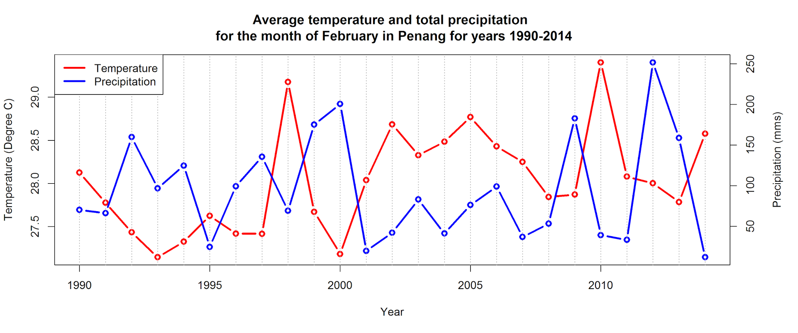
The combination of (dry bulb) air temperatures with data for relative humidity, and wind-speed facilitates the calculation of a ‘heat index’ which is more directly related to ‘human comfort’ than any one of its constituent variables. When the heat index is high the weather will be uncomfortable and, when low, more bearable.  In a previous blog post, we examined average air temperatures and rainfall in Penang suggesting that January and February were the worst times of year to visit Penang since they are usually the hottest and October the best since it is usually coolest. The heat index plotted in the circular plot suggests a slightly different story, however.  April and May have the highest heat indices and are probably potentially the most uncomfortable times of year to visit Penang while the entire period between July and December have similar heat indices.

To produce the plot above, we have again sourced the data from NOAA's National Climatic Data Centre with the hourly dataset coming from the Integrated Surface Database.

We also provide the R code as usual (below) if you would like to produce similar plots for your area of interest.

# Load package libraries
 
library(ggplot2)
library(scales)
library(plyr)
library(dplyr)
library(reshape2)
library(circular)
library(lubridate)
library(grid)
library(zoo)
library(gridExtra)
library(weathermetrics)
library(RColorBrewer)
 
# Setting work directory
 
setwd("d:\\ClimData")
 
# Reading and reformatting raw hourly data downloaded from NCDC
 
dat<-read.table("831677118578dat.txt",header=TRUE,fill=TRUE,na.strings=c("*","**","***","****","*****","******","0.00T*****"))
 
colnames(dat)<-tolower(colnames(dat))
 
Sys.setenv(TZ = "UTC")
dat$dates <- as.POSIXct(strptime(dat$yr..modahrmn,format="%Y%m%d%H%M"))  + 8 * 60 * 60
 
dat$year <- as.numeric(format(dat$dates,"%Y"))
 
dat$month <- as.numeric(format(dat$dates,"%m"))
 
dat$hour<-substring(as.character(dat$dates),12,13)
 
dat$min<-substr(dat$dates,15,16)
 
dat$time<-paste(dat$hour,dat$min,sep=":")
 
dat$tempc <- (dat$temp-32) * (5/9)
 
dat$dewpc <- (dat$dewp-32) * (5/9)
 
dat$tempc[dat$tempc<=10] <- NA
 
dat$tempc[dat$tempc>=40] <- NA
 
dat$dir[dat$dir == 990.0] <- NA 
 
dat$wspd <- (dat$spd)*0.44704
 
# Convert precipitation from inches to mms
 
dat$rain  <- dat$pcp24*25.4
 
# Calculate relative humidity & heat index using weathermetrics package
 
dat$rh <- dewpoint.to.humidity(t = dat$tempc, dp = dat$dewpc, temperature.metric = "celsius")
 
dat$hi <- heat.index(t = dat$tempc,rh = dat$rh,temperature.metric = "celsius",output.metric = "celsius",round = 2)
 
# Commands to reformat dates
 
dat$year <- as.numeric(as.POSIXlt(dat$dates)$year+1900)
dat$month <- as.numeric(as.POSIXlt(dat$dates)$mon+1)
dat$monthf <- factor(dat$month,levels=as.character(1:12),labels=c("Jan","Feb","Mar","Apr","May","Jun","Jul","Aug","Sep","Oct","Nov","Dec"),ordered=TRUE)
dat$weekday <- as.POSIXlt(dat$dates)$wday
dat$weekdayf <- factor(dat$weekday,levels=rev(0:6),labels=rev(c("Mon","Tue","Wed","Thu","Fri","Sat","Sun")),ordered=TRUE)
dat$yearmonth <- as.yearmon(dat$dates)
dat$yearmonthf <- factor(dat$yearmonth)
dat$week <- as.numeric(format(as.Date(dat$dates),"%W"))
dat$hour <- as.numeric(format(strptime(dat$dates, format = "%Y-%m-%d %H:%M"),format = "%H"))
 
dat <- ddply(dat,.(yearmonthf),transform,monthweek=1+week-min(week))
 
# Extract data from 1980 onwards
 
dat1 <- subset(dat, year >= 1980 )
 
# Summarize data for weather variables by hour and month
 
dat2 <- ddply(dat1,.(monthf,hour),summarize, wspd = mean(wspd,na.rm=T))
 
dat3 <- ddply(dat1,.(monthf,hour),summarize, temp = mean(tempc,na.rm=T))
 
dat4 <- ddply(dat1,.(monthf,hour),summarize, hi = mean(hi,na.rm=T))
 
dat6 <- ddply(dat1,.(monthf,hour),summarize, rh = mean(rh,na.rm=T))
 
## Plot Temperature circular Plot
 
p1 = ggplot(dat3, aes(x=monthf, y=hour, fill=temp)) +
  geom_tile(colour="grey70") +
  scale_fill_gradientn(colours = c("#99CCFF","#81BEF7","#FFFFBD","#FFAE63","#FF6600","#DF0101"),name="Temperature\n(Degree C)\n")+
  scale_y_continuous(breaks = seq(0,23),
                     labels=c("12.00am","1:00am","2:00am","3:00am","4:00am","5:00am","6:00am","7:00am","8:00am","9:00am","10:00am","11:00am","12:00pm",
                              "1:00pm","2:00pm","3:00pm","4:00pm","5:00pm","6:00pm","7:00pm","8:00pm","9:00pm","10:00pm","11:00pm")) +
  coord_polar(theta="x") +
  ylab("HOUR OF DAY")+
  xlab("")+
  ggtitle("Temperature")+
  theme(panel.background=element_blank(),
  axis.title.y=element_text(size=10,hjust=0.75,colour="grey20"),
  axis.title.x=element_text(size=7,colour="grey20"),
  panel.grid=element_blank(),
  axis.ticks=element_blank(),
  axis.text.y=element_text(size=5,colour="grey20"),
  axis.text.x=element_text(size=10,colour="grey20",face="bold"),
  plot.title = element_text(lineheight=1.2, face="bold",size = 14, colour = "grey20"),
  plot.margin = unit(c(-0.25,0.1,-1,0.25), "in"),
  legend.key.width=unit(c(0.2,0.2),"in"))
 
p1
 
 
## Plot Wind Speed circular plot
 
p2 = ggplot(dat2, aes(x=monthf, y=hour, fill=wspd)) +
  geom_tile(colour="grey70") +
  scale_fill_gradientn(colours = rev(topo.colors(7)),name="Wind Speed\n(meter/sec)\n")+
  scale_y_continuous(breaks = seq(0,23),
                     labels=c("12.00am","1:00am","2:00am","3:00am","4:00am","5:00am","6:00am","7:00am","8:00am","9:00am","10:00am","11:00am","12:00pm",
                              "1:00pm","2:00pm","3:00pm","4:00pm","5:00pm","6:00pm","7:00pm","8:00pm","9:00pm","10:00pm","11:00pm")) +
  coord_polar(theta="x") +
  ylab("HOUR OF DAY")+
  xlab("")+
  ggtitle("Wind Speed")+
  theme(panel.background=element_blank(),
  axis.title.y=element_text(size=10,hjust=0.75,colour="grey20"),
  axis.title.x=element_text(size=7,colour="grey20"),
  panel.grid=element_blank(),
  axis.ticks=element_blank(),
  axis.text.y=element_text(size=5,colour="grey20"),
  axis.text.x=element_text(size=10,colour="grey20",face="bold"),
  plot.title = element_text(lineheight=1.2, face="bold",size = 14, colour = "grey20"),
  plot.margin = unit(c(-0.25,0.25,-1,0.25), "in"),
  legend.key.width=unit(c(0.2,0.2),"in"))
 
p2
 
 
# Plot Heat Index circular plor
 
p3 = ggplot(dat4, aes(x=monthf, y=hour, fill=hi)) +
  geom_tile(colour="grey70") +
  scale_fill_gradientn(colours = c("#99CCFF","#81BEF7","#FFFFBD","#FFAE63","#FF6600","#DF0101"),name="Temperature\n(Degree C)\n")+
  scale_y_continuous(breaks = seq(0,23),
                     labels=c("12.00am","1:00am","2:00am","3:00am","4:00am","5:00am","6:00am","7:00am","8:00am","9:00am","10:00am","11:00am","12:00pm",
                              "1:00pm","2:00pm","3:00pm","4:00pm","5:00pm","6:00pm","7:00pm","8:00pm","9:00pm","10:00pm","11:00pm")) +
  coord_polar(theta="x") +
  ylab("HOUR OF DAY")+
  xlab("")+
  ggtitle("Heat Index")+
  theme(panel.background=element_blank(),
  axis.title.y=element_text(size=10,hjust=0.75,colour="grey20"),
  axis.title.x=element_text(size=7,colour="grey20"),
  panel.grid=element_blank(),
  axis.ticks=element_blank(),
  axis.text.y=element_text(size=5,colour="grey20"),
  axis.text.x=element_text(size=10,colour="grey20",face="bold"),
  plot.title = element_text(lineheight=1.2, face="bold",size = 14, colour = "grey20"),
  plot.margin = unit(c(-0.5,0.25,-0.25,0.25), "in"),
  legend.key.width=unit(c(0.2,0.2),"in"))
 
p3
 
 
# Plot Relative Humidity circular plor
 
col<-brewer.pal(11,"Spectral")
 
p4 = ggplot(dat6, aes(x=monthf, y=hour, fill=rh)) +
  geom_tile(colour="grey70") +
  scale_fill_gradientn(colours=col,name="Relative Humidity\n(%)\n")+
  scale_y_continuous(breaks = seq(0,23),
                     labels=c("12.00am","1:00am","2:00am","3:00am","4:00am","5:00am","6:00am","7:00am","8:00am","9:00am","10:00am","11:00am","12:00pm",
                              "1:00pm","2:00pm","3:00pm","4:00pm","5:00pm","6:00pm","7:00pm","8:00pm","9:00pm","10:00pm","11:00pm")) +
  coord_polar(theta="x") +
  ylab("HOUR OF DAY")+
  xlab("")+
  ggtitle("Relative Humidity")+
  theme(panel.background=element_blank(),
  axis.title.y=element_text(size=10,hjust=0.75,colour="grey20"),
  axis.title.x=element_text(size=7,colour="grey20"),
  panel.grid=element_blank(),
  axis.ticks=element_blank(),
  axis.text.y=element_text(size=5,colour="grey20"),
  axis.text.x=element_text(size=10,colour="grey20",face="bold"),
  plot.title = element_text(lineheight=1.2, face="bold",size = 14, colour = "grey20"),
  plot.margin = unit(c(-0.5,0.1,-0.25,0.25), "in"),
  legend.key.width=unit(c(0.2,0.2),"in"))
 
p4
 
## Plot and export to png file
 
png(file="Weather_Variables_Circular_Plot.png",width = 12, height = 10, units = "in",
    bg = "white", res = 400, family = "", restoreConsole = TRUE,
    type = "cairo")
 
grid.arrange(p1,p2,p4,p3,nrow=2,main=textGrob("\nWeather Variables by Month and Hour\n(Bayan Lepas Weather Station)",
gp=gpar(fontsize=18,col="grey20",fontface="bold")),sub=textGrob("Source: NOAA National Climatic Data Centre (NCDC)\n",
                                                                                                              gp=gpar(fontsize=9,col="grey20",fontface="italic")))
 
dev.off()

Created by Pretty R at inside-R.org

2014 has seen drought and forest fires on Penang Island

Key point of post

•  February 2014 was the driest since 1990 and in the top 5 warmest

   

 2014 and ‘The Pearl of the Orient’ is looking parched. The grass is brown, the epiphytes that normally festoon the ‘rain’ trees in the Youth Park are wilted, and we’ve even had forest fires in the hills behind the main conurbations (see photos below). Last week aircraft were collecting seawater off Gurney Drive to douse the flames and, according to our friends in Penang, the current dry spell is unprecedented.

Further down south on the steep slopes of Bukit Jambul, there are recurring fires at various patches along the hills. The photo below was taken a few nights ago showing the fires on the hills just behind the Bukit Jambul High School and it has yet to cease entirely since this post was created.

 

As we’ve seen in previous post, while there is some ‘predictable’ seasonality in rainfall on Penang, it is also rather erratic or variable. We’ve plotted daily total rainfall at Penang Airport, below, for 7 selected years, and the first 2 months of 2014. These years give an illustration of some typical patterns. Generally speaking December, January and February are indeed quite dry but this is not always true. January 2000 and February 2005 were, for example, quite wet; early February 2005 seeing greater than 50mms rain in one day.

So what about 2014? There was a bit of rain in mid-January (at least at the airport) but none fell at all in February. Total February rainfall (blue line) since 1990 is plotted below, together with average daily air temperatures for February (red line). February 2014 was the driest for nearly 25 years but not by that much. Februaries 1995 and 2001 were also very dry. [Data for further back in time were available but incomplete records and lines of zeros made us suspect their veracity.]

Perhaps then higher temperatures than usual have exacerbated the low rainfall situation and helped stoke the forest fires? Previously we demonstrated that temperatures have been rising in Penang over the last 20 or so years and the hot period of the year now lasts longer than in the past. February 2014 was pretty hot at around 28.5°C, but nothing like as sweltering as 2010 when a mean temperature of around 29°C was recorded, together with also quite low rainfall.

So what of the connection between temperature and rainfall? The average February temperatures and rainfall 1990-2014 are plotted against each other below. There is obviously a negative relationship between the two (the correlation coefficient = -0.4). Wetter Februaries tend to be cooler and vice-versa.

 

February 2014 has been the driest since 1990 but not the hottest (1998, 2002, 2005, 2010 were all warmer). In summary the relationship between rainfall, temperature, and the triggers for forest fires are complex. Other factors that we have not examined such as humidity and wind speed may also have contributed.

Nevertheless we have shown that February 2014 has been the driest since 1990 on Penang Island and is in the Top 5 warmest years.

As usual, we include the R code we have used to produce the plots in this post. The raw data for these plots however was downloaded from the Global Surface Summary of the Day (GSOD) which is a product developed by the National Climatic Data Centre (NCDC) based in the US. The input data used in building these daily summaries are the Integrated Surface Data (ISD), which includes global data obtained from the USAF Climatology Center, located in the Federal Climate Complex with NCDC. The latest daily summary data are normally available 1-2 days after the date-time of the observations used in the daily summaries.

The datasets can be downloaded from NCDC via a normal web interface at the link below
http://www7.ncdc.noaa.gov/CDO/cdoselect.cmd?datasetabbv=GSOD

or through their FTP site at the following link

ftp://ftp.ncdc.noaa.gov/pub/data/gsod

# Setting work directory
 
setwd("d:\\ClimData")
 
list.files()
 
# Reading and reformatting raw data downloaded from NCDC
 
dat<-read.table("CDO2812586929956.txt",header=F,skip=1)
 
colnames(dat)<-c("stn","wban","yearmoda","temp","tempc","dewp","dewpc","slp","slpc","stp","stpc","visib","visibc","wdsp","wdspc","mxspd","gust","maxtemp","mintemp","prcp","sndp","frshtt")
 
dat$yearmoda <- strptime(dat$yearmoda,format="%Y%m%d")
 
min.date <- min(dat$yearmoda)
max.date <- max(dat$yearmoda)
 
dat$prcp <- as.character(dat$prcp)
dat$prcp1<- as.numeric(substr(dat$prcp,1,4))
dat$prcpflag <- substr(dat$prcp,5,5)
 
dat$rain  <- dat$prcp1*25.4
dat$tempdc <- (dat$temp-32) * (5/9)
 
dat$rain[dat$rain > 1000 ] <- NA
 
dat$year <- as.numeric(format(dat$yearmoda,"%Y"))
dat$month <- as.numeric(format(dat$yearmoda,"%m"))
dat$day <- as.numeric(format(dat$yearmoda,"%d"))
 
# Plotting precipitation for various years in Penang from daily precipitation data
 
library(ggplot2)
library(scales)
 
dat$date<-as.Date(dat$yearmoda)
 
datsub <- subset(dat, year == 1990 | year == 1995 | year == 2000 | year == 2005 | year == 2010 | year == 2012 | year ==2013 | year == 2014)
 
dat1 <- transform(datsub, date = as.Date(paste(2000, month, day, sep="/")))
 
boxplot.title = 'Precipitation in Penang'
boxplot.subtitle = 'Data source : Federal Climate Complex, Global Surface Summary Of Day Data Version 7'
 
g <- ggplot(dat1, aes(date, rain)) +
  geom_line(col="blue", size=0.65) + 
  facet_wrap( ~ year, ncol = 2) +
  xlab("") + ylab("Precipitation (mms)") +
  scale_x_date(label = date_format("%b"), breaks = seq(min(dat1$date), max(dat1$date), "month")) +
  scale_y_continuous(limits = c(0,150)) +
  ggtitle(bquote(atop(.(boxplot.title), atop(italic(.(boxplot.subtitle)), "")))) + theme(plot.title = element_text(face = "bold",size = 16,colour="black")) +
  theme(legend.position = "none") + theme_bw()
g
 
ggsave(g, file="Penang_GSOD_Prcp_Plots.png", width=10, height=7)
 
# Plotting Average monthly temperature and total precipitation
 
avgtemp <- aggregate(tempdc ~ year + month, data = dat, FUN = mean)
totrain <- aggregate(rain ~ year + month, data = dat, FUN = sum)
 
avgtempfeb <- subset(avgtemp, month == 2 & year >= 1990)
totrainfeb <- subset(totrain, month == 2 & year >= 1990)
 
par(mar=c(5,4,4,5)+.1)
plot(avgtempfeb$year,avgtempfeb$tempdc,type="b",col="red",lwd=3,xlab="",ylab="")
par(new=TRUE)
plot(avgtempfeb$year,totrainfeb$rain,,type="b",col="blue",lwd=3,xaxt="n",yaxt="n",xlab="Year",ylab="Temperature (Degree C)",
     main = "Average temperature and total precipitation \n for the month of February in Penang for years 1990-2014")
axis(4)
mtext("Precipitation (mms)",side=4,line=3)
abline(v=1949:2014,lty=3,col='grey70')
legend("topleft",col=c("red","blue"),lwd=3,legend=c("Temperature","Precipitation"))
 
dev.off()
 
# Plot correlation between average temperature and total precipitation
 
png(filename = "Penang_TempPrcp_Correlation_Years_1990-2014.png",height=5,width=10,
    bg = "white",units='in', res = 300, family = "", restoreConsole = TRUE,
    type = "windows")
 
reg <- lm(totrainfeb$rain~avgtempfeb$tempdc)
plot(avgtempfeb$tempdc,totrainfeb$rain,type='n',xlab="Temperature (Degree C)",ylab="Precipitation (mms)",
     main = "Correlation between average temperature and total precipitation \n for the month of February in Penang for years 1990-2014")
 
abline(v=c(27.5,28,28.5,29,29.5,30),lty=3,col='grey70')
abline(h=c(0,50,100,150,200.250,300),lty=3,col='grey70')
text(avgtempfeb$tempdc,totrainfeb$rain,as.character(totrainfeb$year),cex=1.2,col="red")
box(lty = "solid", col = 'black',lwd=3)
 
# Correlation value between total precipitation and temperatures
 
cor(totrainfeb$rain,avgtempfeb$tempdc)
 
dev.off()

Created by Pretty R at inside-R.org